
Converting a large CSV to a Delta Table and comparing the size
A hands-on demo.

This is the second article in the series on Delta Lake storage.
Part 1 talked about what Delta Tables are and why they’re ideal for long-term archiving
A hands-on demo: converting a large CSV to a Delta Table and comparing the size ← you’re here
Querying Delta Tables with DuckDB, no Spark required
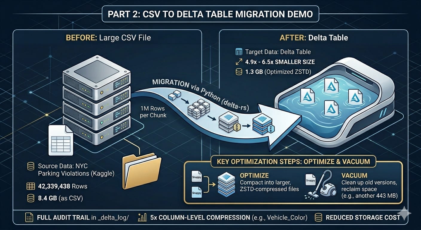
I wanted a dataset big enough to feel real. Something closer to what actually accumulates in a production database over a few years. We’ll be using the NYC Parking Violations dataset from Kaggle. It contains four fiscal years of parking tickets issued across New York City.
42,339,438 rows
8.4 GB as a CSV
That felt like enough to work with.
The Migration
I used delta-rs, the Python package, to write the data to a local Delta Table. No Spark, no cluster. Just Python reading the CSV in chunks and writing it out as Parquet files within the Delta Table format.
The full code is in the companion repo here. The README.md file has instructions to follow along.
import pandas as pd
import pyarrow as pa
from deltalake import write_deltalake

CHUNKSIZE = 1_000_000
first = True

for chunk in pd.read_csv("data/nyc_parking_violations.csv", chunksize=CHUNKSIZE, dtype=str):
    chunk.columns = [c.replace(" ", "_").replace("/", "_") for c in chunk.columns]
    table = pa.Table.from_pandas(chunk, preserve_index=False)
    write_deltalake("data/delta_table", table, mode="overwrite" if first else "append", schema_mode="merge")
    first = False
The script reads a million rows at a time, writes to Delta, and repeats until done.
What do the numbers say
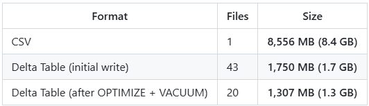
The delta table was 4.9x smaller on the first write, and 6.5x after running a couple of extra steps.
The initial write produces one Parquet file per chunk. 43 Snappy-compressed files in this case. Running OPTIMIZE compacts those into fewer, larger files and rewrites them using ZSTD compression, which squeezes them down further. VACUUM then cleans up the old Snappy versions. Together they saved another 443 MB.
from deltalake import DeltaTable
dt = DeltaTable("data/delta_table")
dt.optimize.compact()
dt.vacuum(retention_hours=0, enforce_retention_duration=False, dry_run=False)
Dictionary Encoding
Where Parquet shines is when you have columns with repeated values. It applies a concept called Dictionary Encoding automatically, when the ratio of unique values to total rows is low enough to make it worthwhile. A colour column with 5,745 unique values across 42 million rows is a perfect candidate. A column of unique transaction IDs is not.
In this case, we will take the column Vehicle_Color as an example.
Across 42 million rows, there are only 5,745 unique colour values (5,745 unique colours? — clearly a free-text field?!). Things like WHITE, BLACK, GREY, BLK, GY. In a CSV, every row stores the full string. In Parquet, each unique value is stored once in a dictionary, and each row just stores a small integer pointing to it.
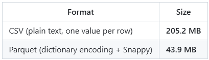
5x smaller on a single column.
A Note on the Delta Log
You may ask if Parquet does all the heavy lifting why store data in a delta table format. The Delta Table format is what maintains ACID compliance. It keeps track of all the changes to the table from the time when it was created. When you look at the Delta Table folder after running everything, you’ll see this:
data/delta_table/
├── _delta_log/
│   ├── 00000000000000000000.json   ← WRITE (overwrite, chunk 1, 1M rows)
│   ├── 00000000000000000001.json   ← WRITE (append, chunk 2, 1M rows)
│   ├── ...                         ← WRITE (append, chunks 3-42)
│   ├── 00000000000000000043.json   ← OPTIMIZE (43 files to 20 files)
│   ├── 00000000000000000044.json   ← VACUUM START (43 files to delete)
│   └── 00000000000000000045.json   ← VACUUM END (completed)
├── part-00000-c6e7a34b-...zstd.parquet
├── part-00000-bc09554a-...zstd.parquet
└── ...
Opening the early log entries, you’ll find snappy.parquet in the add records. That’s the initial write using Snappy compression by default. In the OPTIMIZE entry, you’ll find those replaced with .zstd.parquet files. Snappy is the default in most tools because it’s fast to read and write. ZSTD trades a bit of compute for better compression ratios, making it a better fit for files you’re storing long term and reading less frequently. The Parquet docs cover the full list of supported codecs if you want to go deeper.
Each JSON entry records exactly what happened: which files were added, which were removed, how many rows, min/max values per column. Here’s what a single append entry looks like:
{ "commitInfo": { "operation": "WRITE", "operationParameters": { "mode": "Append" },
    "operationMetrics": { "num_added_files": 1, "num_added_rows": 1000000 } } }
{ "add": { "path": "part-00000-27e284b6-...snappy.parquet", "size": 36893533,
    "stats": { "numRecords": 1000000,
      "minValues": { "Issue_Date": "01/01/2013", ... },
      "maxValues": { "Issue_Date": "12/25/2013", ... },
      "nullCount": { "Vehicle_Make": 5589, ... } } } }
And here’s what the OPTIMIZE entry looks like:
{ "commitInfo": { "operation": "OPTIMIZE",
    "operationMetrics": {
      "numFilesAdded": 20,
      "numFilesRemoved": 43,
      "filesAdded":   { "totalFiles": 20, "totalSize": 1370418125 },
      "filesRemoved": { "totalFiles": 43, "totalSize": 1834829450 } } } }
{ "remove": { "path": "part-00000-357b4b21-...snappy.parquet", "size": 51763870 } }
{ "add":    { "path": "part-00000-c6e7a34b-...zstd.parquet",   "size": 77495774,
    "stats": { "numRecords": 2000000, ... } } }
43 small Snappy files compacted into 20 larger ZSTD files. Total size dropped from 1.83 GB to 1.37 GB.
And once VACUUM runs:
{ "commitInfo": { "operation": "VACUUM START",
    "operationMetrics": { "numFilesToDelete": 43, "sizeOfDataToDelete": 1834829450 } } }
{ "commitInfo": { "operation": "VACUUM END",
    "operationParameters": { "status": "COMPLETED" },
    "operationMetrics": { "numDeletedFiles": 43 } } }
43 files, 1.75 GB reclaimed.
It’s a complete audit trail. Every operation, in order, with the numbers to back it up. In a future post I will write in detail about how you can infer more information from these json files using a function built within delta_rs.
Bringing It Back to the Cost
The numbers here are for a CSV, not a SQL Server table. I don’t have a SQL Server instance that can hold 43 million rows for free, but I’m planning to do that comparison in a future post. But the point from Part 1 still stands. SQL Server stores data row by row, adds index overhead, and keeps an instance running whether you’re querying or not.
The same 42 million rows that sit in 1.3 GB as a Delta Table would take up considerably more in a relational database and cost you more to keep around. For data that gets queried occasionally, that overhead is hard to justify.
What’s Next
Part 3: querying this Delta Table with DuckDB. No Spark, no cluster. Just SQL on your laptop against 42 million rows. I hope this series has been helpful. Please subscribe if you want to be notified for the future posts. I will add an additional post to this series to show how the above example works the same way in a cost effective object storage like ADLS. See you soon.